In light of word embeddings’ recent popularity, I’ve been playing around with a version called Latent Semantic Analysis (LSA). Admittedly, LSA has fallen out of favor with the rise of neural embeddings like Word2Vec, but there are several virtues to LSA including decades of study by linguists and computer scientists. (For an introduction to LSA for humanists, I highly recommend Ted Underwood’s post “LSA is a marvelous tool, but…“.) In reality, though, this blog post is less about LSA and more about tinkering with it and using it for parts.
Like other word embeddings, LSA seeks to learn about words’ semantics by way of context. I’ll sidestep discussion of LSA’s specific mechanics by saying that it uses techniques that are closely related to ones commonly used in distant reading. Broadly, LSA constructs something like a document-term matrix (DTM) and then performs something like Principle Component Analysis (PCA) on it.1 (I’ll be using those later in the post.) The art of LSA, however, lies in between these steps.
Typically, after constructing a corpus matrix, LSA involves some kind of weighting of the raw word counts. The most familiar weight scheme is (l1) normalization: sum up the number of words in a document and divide the individual word counts, so that each cell in the matrix represents a word’s relative frequency. This is something distant readers do all the time. However, there is an extensive literature on LSA devoted to alternate weights that improve performance on certain tasks, such as analogies or document retrieval, and on different types of documents.
This is the point that piques my curiosity. Can we use different weightings strategically to capture valuable features of a textual corpus? How might we use a semantic model like LSA in existing distant reading practices? The similarity of LSA to a common technique (i.e. PCA) for pattern finding and featurization in distant reading suggests that we can profitably apply its weight schemes to work that we are already doing.
What follows is naive empirical observation. No hypotheses will be tested! No texts will be interpreted! But I will demonstrate the impact that alternate matrix weightings have on the patterns we identify in a test corpus. Specifically, I find that applying LSA-style weights has the effect of emphasizing textual subject matter which correlates strongly with diachronic trends in the corpus.
I resist making strong claims about the role that matrix weighting plays in the kinds of arguments distant readers have made previously — after all, that would require hypothesis testing — however, I hope to shed some light on this under-explored piece of the interpretive puzzle.
Matrix Weighting
Matrix weighting for LSA gets broken out into two components: local and global weights. The local weight measures the importance of a word within a given text, while the global weight measures the importance of that word across texts. These are treated as independent functions that multiply one another.

where i refers to the row corresponding to a given word and j refers to the column corresponding to a given text.2 One common example of such a weight scheme is tf-idf, or term frequency-inverse document frequency. (Tf-idf has been discussed for its application to literary study at length by Stephen Ramsey and others.)
Research on LSA weighting generally favors measurements of information and entropy. Typically, term frequencies are locally weighted using a logarithm and globally weighted by measuring the term’s entropy across documents. How much information does a term contribute to a document? How much does the corpus attribute to that term?
While there are many variations of these weights, I have found one of the most common formulations to be the most useful on my toy corpus.3


where tf is the raw count of words in a document, p is the conditional probability of a document given a word, and N is the total number of documents in the corpus. For the global weights, I used normalized (l1) frequencies for each term when calculating the probabilities (pi,j). This prevents longer texts from having disproportionate influence on the term’s entropy. Vector (l2) normalization is applied over each document, after weights have been applied.
To be sure, this is not the only weight and normalization procedure one might wish to use. The formulas above merely describe the configuration I have found most satisfying (so far) on my toy corpus. Applying variants of those formulas on new data sets is highly encouraged!
Log-Entropy vs. Relative Frequency
My immediate goal for this post is to ask what patterns get emphasized by log-entropy weighting a DTM. Specifically, I’m asking what gets emphasized when we perform a Principle Component Analysis, however the fact of modeling feature variance suggests that the results may have bearing on further statistical models. We can do this at a first approximation by comparing the results from log-entropy to those of vanilla normalization. To this end, I have pulled together a toy corpus of 400 twentieth-century American novels. (This sample approximates WorldCat holdings, distributed evenly across the century.)
PCA itself is a pretty useful model for asking intuitive questions about a corpus. The basic idea is that it looks for covariance among features: words that appear in roughly the same proportions to one another (or inversely) across texts probably indicate some kind of interesting subject matter. Similarly, texts that contain a substantive share of these terms may signal some kind of discourse. Naturally, there will be many such clusters of covarying words, and PCA will rank each of these by the magnitude of variance they account for in the DTM.
Below are two graphs that represent the corpus of twentieth-century novels. Each novel appears as a circle, while the color indicates its publication date: the lightest blue corresponds to 1901 and the brightest purple to 2000. Note that positive/negative signs are assigned arbitrarily, so that, in Fig. 1, time appears to move from the lower-right hand corner of the graph to the upper-left.
To produce each graph, PCA was performed on the corpus DTM. The difference between graphs consists in the matrices’ weighting and normalization. To produce Fig. 2, the DTM of raw word counts was (l1) normalized by dividing all terms by the sum of the row. On the other hand, Fig. 1 was produced by weighting the DTM according to the log-entropy formula described earlier. Note that stop words were not removed from either DTM.4

Figure 1. Log-Entropy Weighted DTM.
Explained Variance: PC 1 (X) 2.8%, PC 2 (Y) 1.8%
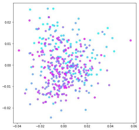
Figure 2. Normalized DTM.
Explained Variance: PC 1 (X) 25%, PC 2 (Y) 10%
The differentiation between earlier and later novels is visibly greater in Fig. 1 than Fig. 2. We can gauge that intuition formally, as well. The correlation between these two principle components and publication year is substantial, r2 = 0.49. Compare that to Fig. 2, where r2 = 0.07. For the log-entropy matrix, the first two principle components encode a good deal of information about the publication year, while those of the other matrix appear to capture something more synchronic.5
Looking at the most important words for the first principle component of each graph (visualized as the x-axis; accounting for the greatest variance among texts in the corpus) is pretty revealing about what’s happening under the hood. Table 1 and Table 2 show the top positive and negative words for the first principle component from each analysis. Bear in mind that these signs are arbitrary and solely indicate that words are inversely proportional to one another.
|
|
||||||||||||||||||||||||||||||||||||||||||||||||
The co-varying terms in the log-entropy DTM in Table 1 potentially indicate high level differences in social milieu and genre. Among the positive terms, we find British spelling and self-consciously literary diction. (Perhaps it is not surprising that many of the most highly ranked novels on this metric belong to Henry James.) The negative terms, conversely, include informal spelling and word choice. Similarly, the transition from words like carriage and madame to phone and cops gestures toward changes that we might expect in fiction and society during the twentieth century.
Although I won’t describe them at length, I would like to point out that the second principle component (y-axis) is equally interesting. The positive terms refer to planetary conflict, and the cluster of novels at the top of the graph comprise science fiction. The inverse terms include familial relationships, common first names, and phonetic renderings of African American Vernacular English (AAVE). (It is telling that some of the novels located furthest in that direction are those of Paul Laurence Dunbar.) This potentially speaks to ongoing conversations about race and science fiction.
On the other hand, the top ranking terms in Table 2 for the vanilla-normalized DTM are nearly all stop words. This makes sense when we remember that they are the most frequent words by far in a typical text. By their sheer magnitude, any variation in these common words will constitute a strong signal for PCA. Granted, stop words can be easily removed during pre-processing of texts. However, this means a trade-off for the researcher, since they are known to encode valuable textual features like authorship or basic structure.
The most notable feature of the normalized DTM’s highly ranked words is the inverse relationship between gendered pronouns. Novels about she and her tend to speak less about he and his, and vice versa. The other words in the list don’t give us much of an interpretive foothold on the subject matter of such novels, however we can find a pattern in terms of the metadata: the far left side of the graph is populated mostly by women-authored novels and the far right by men. PCA seems to be performing stylometry and finding substantial gendered difference. This potentially gestures toward the role that novels play as social actors, part of a larger cultural system that reproduces gendered categories.
This is a useful finding in and of itself, however, looking at further principle components of the normalized DTM reveals the limitation of simple normalization. The top ranking words for next several PCs are comprised of the same stop words but in different proportions. PCA is simply accounting for stylometric variation. Again, it is easy enough to remove stop words from the corpus before processing. Indeed, removing stop words reveals an inverse relationship between dialogue and moralizing narrative.6 Yet, even with a different headline pattern, one finds oneself in roughly the same position. The first several PCs articulate variations of the most common words. The computer is more sensitive to patterns among words with relatively higher frequency, and Zipf’s Law indicates that some cluster of words will always rise to the top.
Conclusion
From this pair of analyses, we can see that our results were explicitly shaped by the matrix weighting. Log-entropy got us closer to the subject matter of the corpus, while typical normalization captures more about authorship (or basic textual structure, when stop words are removed). Each of these is attuned to different but equally valuable research questions, and the selection of matrix weights will depend on the category of phenomena one hopes to explore.
I would like to emphasize that it is entirely possible that the validity of these findings is limited to applications of PCA. Log-entropy was chosen here because it optimizes semantic representation on a PCA-like model. Minimally, we may find it useful when we are looking specifically at patterns of covariance or even when using the principle components as features in other models.
However, this points us to a larger discussion about the role of feature representation in our modeling. As a conceptual underpinning, diction takes us pretty far toward justifying the raw counts of words that make up a DTM. (How often did the author choose this word?) But it is likely that we wish to find patterns that do not reduce to diction alone. The basis of a weight scheme like log-entropy in information theory moves us to a different set of questions about representating a text to the computer. (How many bits does this term contribute to the novel?)
The major obstacle then is not a technical one but interpretive. Information theory frames the text as a message that has been stored and transmitted. The question this raises, then: what else is a novel, if not a form of communication?
Footnotes
1. In reality, LSA employs a term-context matrix, that turns the typical DTM on its side: rows correspond unique terms in the corpus and columns to documents (or another unit that counts as “context,” such as a window of adjacent words). After weighting and normalizing the matrix, LSA performs a Singular Value Decomposition (SVD). PCA is an application of SVD.
2. Subscripts i and j correspond to the rows and columns of the term-context matrix described in fn. 1, rather than the document-term matrix that I will use later.
3. This formulation appears, for example in Nakov et al (2001) and Pincombe (2004). I have tested variations of these formulas semi-systematically, given the corpus and pre-processing. This pair of local and global weights were chosen because they resulted in principle components that correlated most strongly with publication date, as described in the next section. It was also the case that weight schemes tended to minimize the role of stop words in rough proportion to that correlation with date. The value of this optimization is admittedly more intuitive than formal.
For the results of other local and global weights, see the Jupyter Notebook in the GitHub repo for this post.
4. This is an idiosyncratic choice. It is much more common to remove stop words in both LSA specifically and distant reading generally. At bottom, the motivation to keep them is to identify baseline performance for log-entropy weighting, before varying pre-processing procedures. In any case, I have limited my conclusions to ones that are valid regardless of stop word removal.
Note also that about the most common 12,000 tokens were used in this model, or accounting for 95% of the total words in the corpus. Reducing that number to the most common 3,000 tokens, or about 80% of total words, did not appreciably change the results reported in this post.
5. When stop words were removed, log-entropy performed slightly worse on this metric (r2 = 0.48), while typical normalization performed slightly better (r2 = 0.10). The latter result is consistent with the overall trend that minimizing stop words improves correlation with publication date. However, the negative effect on log-entropy suggests that it is able to leverage valuable information encoded in stop words, even while the model is not dominated by them.
6. See Table 3 below for list of top ranked words in first principle component when stop words are removed from the normalized DTM. Note that, for log-entropy, removing stop words does not substantially change its list of top words.
| Table 3: Normalized DTM, stopwords removed | |
| Positive | Negative |
| said | great |
| don | life |
| got | world |
| didn | men |
| know | shall |
| ll | young |
| just | day |
| asked | new |
| looked | long |
| right | moment |

One thought on “A Naive Empirical Post about DTM Weighting”